Churn Prediction with Telecommunication Data
This project serves as an example of the baseline_optimal.class_task module application.
0. Dependencies
[2]:
import pandas as pd
import matplotlib.pyplot as plt
from sklearn.model_selection import train_test_split
from sklearn.preprocessing import LabelEncoder
from baseline_optimal import ClassTask

%matplotlib inline
import warnings
warnings.filterwarnings('ignore')
Neat and clean import.
1. Problem Statement
The dataset used for this project is synthetic from a telecommunications mobile phone carrier which can be found through this AWS Machine Learning Blog.
In the blog, the synthetic dataset is used as an example to showcase the power of Amazon SageMaker Canvas, which provides a simple interface that allows users to build a customer churn machine learning model without any programming.
The blog states that the model could score a 97.9% accuracy on this synthetic dataset at its best. Through this project, we want to explore:
Can we obtain a machine learning pipeline that achieves a higher score?
Which features are the most influencial in determining whether a customer will churn?
2. Data Collection
Data source: AWS Machine Learning Blog
The synthetic dataset contains 5000 observations with 21 variables.
Load the data:
[3]:
df = pd.read_csv("../data/churn.csv")
Display the first 5 observations:
[ ]:
df.head()
| State | Account Length | Area Code | Phone | Int'l Plan | VMail Plan | VMail Message | Day Mins | Day Calls | Day Charge | ... | Eve Calls | Eve Charge | Night Mins | Night Calls | Night Charge | Intl Mins | Intl Calls | Intl Charge | CustServ Calls | Churn? | |
|---|---|---|---|---|---|---|---|---|---|---|---|---|---|---|---|---|---|---|---|---|---|
| 0 | PA | 163 | 806 | 403-2562 | no | yes | 300 | 8.162204 | 3 | 7.579174 | ... | 4 | 6.508639 | 4.065759 | 100 | 5.111624 | 4.928160 | 6 | 5.673203 | 3 | True. |
| 1 | SC | 15 | 836 | 158-8416 | yes | no | 0 | 10.018993 | 4 | 4.226289 | ... | 0 | 9.972592 | 7.141040 | 200 | 6.436188 | 3.221748 | 6 | 2.559749 | 8 | False. |
| 2 | MO | 131 | 777 | 896-6253 | no | yes | 300 | 4.708490 | 3 | 4.768160 | ... | 3 | 4.566715 | 5.363235 | 100 | 5.142451 | 7.139023 | 2 | 6.254157 | 4 | False. |
| 3 | WY | 75 | 878 | 817-5729 | yes | yes | 700 | 1.268734 | 3 | 2.567642 | ... | 5 | 2.333624 | 3.773586 | 450 | 3.814413 | 2.245779 | 6 | 1.080692 | 6 | False. |
| 4 | WY | 146 | 878 | 450-4942 | yes | no | 0 | 2.696177 | 3 | 5.908916 | ... | 3 | 3.670408 | 3.751673 | 250 | 2.796812 | 6.905545 | 4 | 7.134343 | 6 | True. |
5 rows × 21 columns
Definitions of independent and dependent variables:
Features:
State- The US state in which the customer resides, indicated by a two-letter abbreviationAccount Length– The number of days that this account has been activeArea Code– The three-digit area code of the customer’s phone numberPhone– The remaining seven-digit phone numberInt’l Plan– Whether the customer has an international calling plan (yes/no)VMail Plan– Whether the customer has a voice mail feature (yes/no)VMail Message– The average number of voice mail messages per monthDay Mins– The total number of calling minutes used during the dayDay Calls– The total number of calls placed during the dayDay Charge– The billed cost of daytime callsEve Mins, Eve Calls, Eve Charge– The billed cost for evening callsNight Mins, Night Calls, Night Charge– The billed cost for nighttime callsIntl Mins, Intl Calls, Intl Charge– The billed cost for international callsCustServ Calls– The number of calls placed to customer service
Target:
Churn?– Whether the customer left the service (true/false)
3. Exploratory Data Analysis
You know how to do this - we’ll just check the target class distribution:
[8]:
labels = ['Not Churned', 'Churned']
sizes = df['Churn?'].value_counts()
explode = [0, 0.1]

fig, ax = plt.subplots()
ax.pie(sizes, explode=explode, labels=labels, autopct='%1.1f%%',
       shadow=True, startangle=90)
plt.title(label='Target Class Distribution')
plt.show()
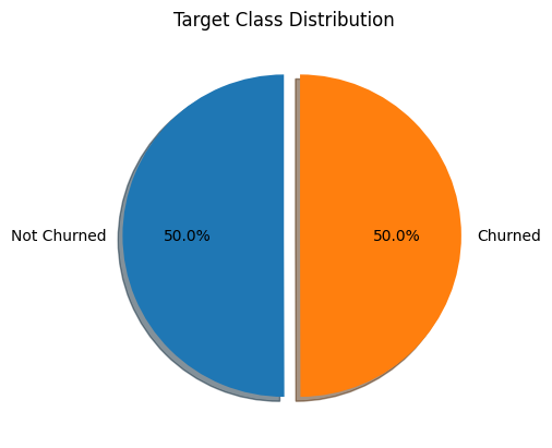
The target class is perfectly balanced.
4. Data Preparation
We remove Area Code, Phone, and State from the data.
The we separate the features and the target:
[9]:
drop = ['Area Code', 'Phone', 'State', 'Churn?']
X = df.drop(drop, axis=1)
y = df['Churn?']
Split the training and the test data given ratio 4:1:
[10]:
X_train, X_test, y_train, y_test = train_test_split(X, y, test_size=0.2, random_state=123)
Encode the target data as some classifier implementations don’t support categorical data:
[11]:
t_e = LabelEncoder()
y_train = t_e.fit_transform(y_train)
y_test = t_e.transform(y_test)
Minimum efforts on preprocessing the data.
5. Optimization and Results
Create a ClassTask object:
[12]:
task = ClassTask()
Search for the optimal pipeline:
[13]:
task.optimize(X_train, y_train)
The evaluation metric is set as accuracy by default. The best cross validation score is 0.95 on the training data:
[14]:
task.best_score
[14]:
0.94875
Get probability estimates using the test data:
[17]:
pred_prob = task.predict(X_test)
Get performance scores on the test data:
[18]:
scores = task.evaluate(X_test, y_test)
scores
[18]:
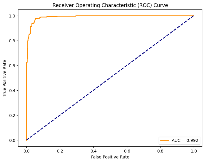
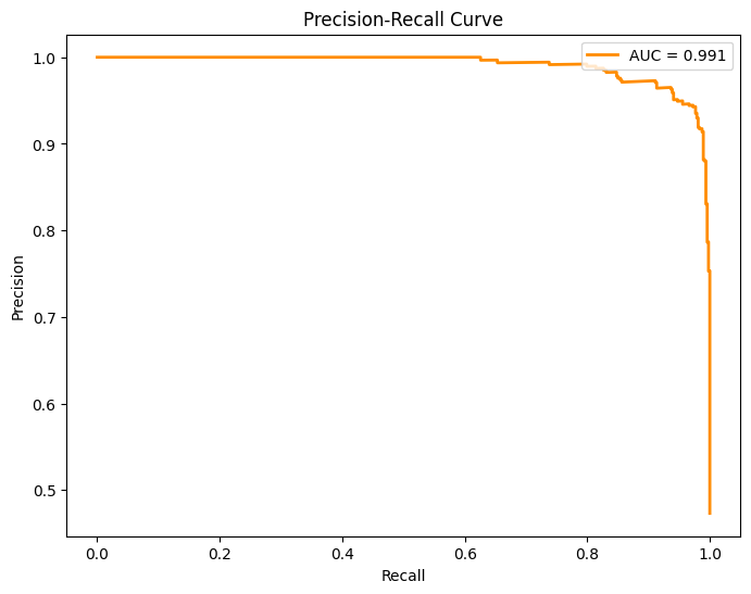
| AUC-ROC | Accuracy | Average Precision | Recall | Precision | F1 | |
|---|---|---|---|---|---|---|
| 0 | 0.992 | 0.961 | 0.991 | 0.977 | 0.943 | 0.96 |
The optimal pipeline has promising performances across all measures.
Obtain the best imblearn.pipeline.Pipeline object:
[19]:
best_pipeline = task.best_pipeline
Use imblearn.pipeline.Pipeline API to get the processing pipeline as well as the estimator:
[20]:
best_processor = best_pipeline.named_steps['processor']
best_estimator = best_pipeline.named_steps['estimator']
See how the training data is processed and transformed in the optimal pipeline:
[21]:
best_processor
[21]:
ColumnTransformer(transformers=[('numerical_pipeline',
                                 Pipeline(steps=[('numerical_imputer',
                                                  SimpleImputer(fill_value=-1)),
                                                 ('scaler', MinMaxScaler())]),
                                 ['Account Length', 'VMail Message', 'Day Mins',
                                  'Day Calls', 'Day Charge', 'Eve Mins',
                                  'Eve Calls', 'Eve Charge', 'Night Mins',
                                  'Night Calls', 'Night Charge', 'Intl Mins',
                                  'Intl Calls', 'Intl Charge',
                                  'CustServ Calls']),
                                ('categorical_pipeline',
                                 Pipeline(steps=[('categorical_imputer',
                                                  SimpleImputer(fill_value='missing',
                                                                strategy='most_frequent')),
                                                 ('encoder',
                                                  OneHotEncoder(drop='first'))]),
                                 ["Int'l Plan", 'VMail Plan'])])
In a Jupyter environment, please rerun this cell to show the HTML representation or trust the notebook. On GitHub, the HTML representation is unable to render, please try loading this page with nbviewer.org.
ColumnTransformer(transformers=[('numerical_pipeline',
                                 Pipeline(steps=[('numerical_imputer',
                                                  SimpleImputer(fill_value=-1)),
                                                 ('scaler', MinMaxScaler())]),
                                 ['Account Length', 'VMail Message', 'Day Mins',
                                  'Day Calls', 'Day Charge', 'Eve Mins',
                                  'Eve Calls', 'Eve Charge', 'Night Mins',
                                  'Night Calls', 'Night Charge', 'Intl Mins',
                                  'Intl Calls', 'Intl Charge',
                                  'CustServ Calls']),
                                ('categorical_pipeline',
                                 Pipeline(steps=[('categorical_imputer',
                                                  SimpleImputer(fill_value='missing',
                                                                strategy='most_frequent')),
                                                 ('encoder',
                                                  OneHotEncoder(drop='first'))]),
["Int'l Plan", 'VMail Plan'])])['Account Length', 'VMail Message', 'Day Mins', 'Day Calls', 'Day Charge', 'Eve Mins', 'Eve Calls', 'Eve Charge', 'Night Mins', 'Night Calls', 'Night Charge', 'Intl Mins', 'Intl Calls', 'Intl Charge', 'CustServ Calls']
SimpleImputer(fill_value=-1)
MinMaxScaler()
["Int'l Plan", 'VMail Plan']
SimpleImputer(fill_value='missing', strategy='most_frequent')
OneHotEncoder(drop='first')
The optimal estimator is a XGBClassifier object:
[22]:
best_estimator
[22]:
XGBClassifier(base_score=None, booster=None, callbacks=None,
              colsample_bylevel=None, colsample_bynode=None,
              colsample_bytree=None, device=None, early_stopping_rounds=None,
              enable_categorical=False, eval_metric=None, feature_types=None,
              gamma=None, grow_policy=None, importance_type=None,
              interaction_constraints=None, learning_rate=0.08044551460612077,
              max_bin=None, max_cat_threshold=None, max_cat_to_onehot=None,
              max_delta_step=None, max_depth=10, max_leaves=None,
              min_child_weight=None, missing=nan, monotone_constraints=None,
              multi_strategy=None, n_estimators=249, n_jobs=None,
              num_parallel_tree=None, random_state=123, ...)
In a Jupyter environment, please rerun this cell to show the HTML representation or trust the notebook. On GitHub, the HTML representation is unable to render, please try loading this page with nbviewer.org.
XGBClassifier(base_score=None, booster=None, callbacks=None,
              colsample_bylevel=None, colsample_bynode=None,
              colsample_bytree=None, device=None, early_stopping_rounds=None,
              enable_categorical=False, eval_metric=None, feature_types=None,
              gamma=None, grow_policy=None, importance_type=None,
              interaction_constraints=None, learning_rate=0.08044551460612077,
              max_bin=None, max_cat_threshold=None, max_cat_to_onehot=None,
              max_delta_step=None, max_depth=10, max_leaves=None,
              min_child_weight=None, missing=nan, monotone_constraints=None,
              multi_strategy=None, n_estimators=249, n_jobs=None,
              num_parallel_tree=None, random_state=123, ...)
Plot the ROC curve:
[23]:
task.plot_roc_curve(X_test, y_test)
Plot the PR curve:
[24]:
task.plot_pr_curve(X_test, y_test)
Plot the confusion matrix:
[25]:
task.plot_confusion_matrix(X_test, y_test)
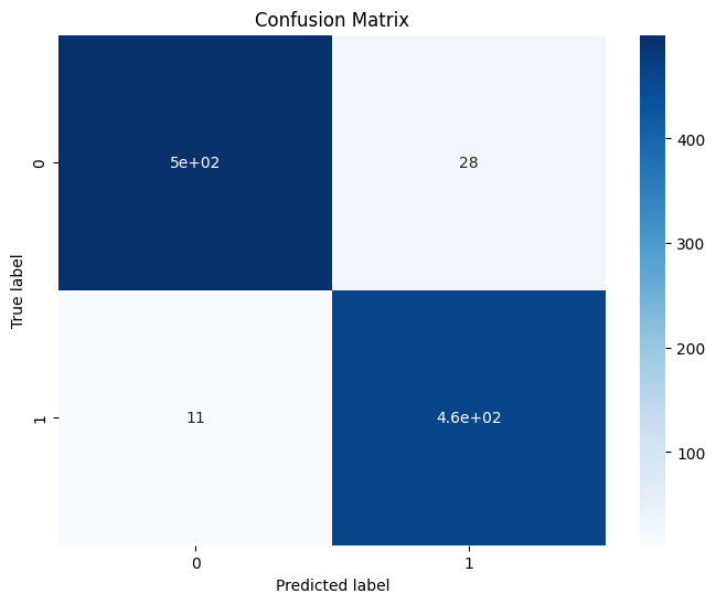
We barely see misclassified instances.
Note that because we didn’t set select=True in the optimize function, all features are considered. Plot feature importances based on Shapley values:
[26]:
task.plot_feature_importances(X_test)
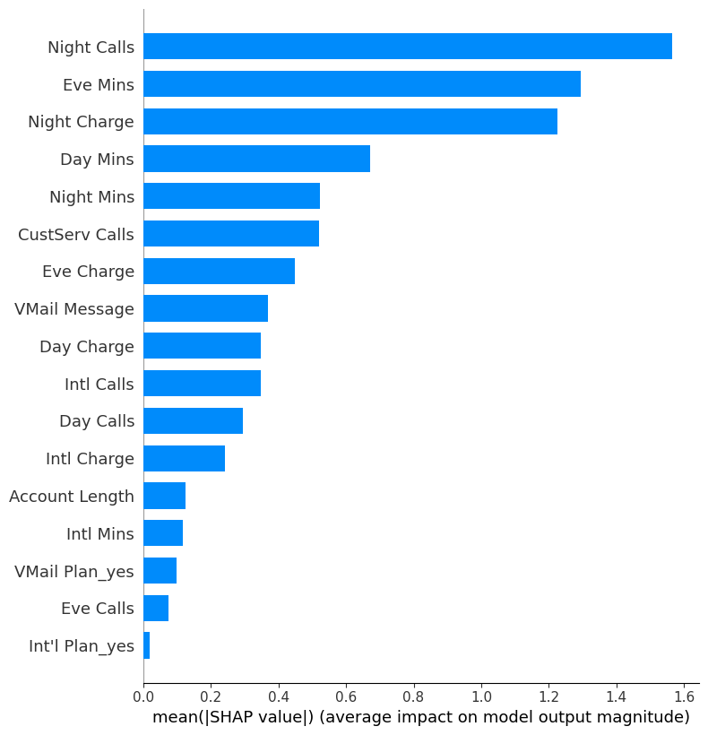
The SHAP values are telling us that on average, Night Calls, Eve Mins, and Night Charge are the most important features contributing to the predictions.
Meanwhile, Int'l Plan_yes is weighted the least.
Next, visualize the directionality impact of the features:
[28]:
task.plot_feature_directionality(X_test)
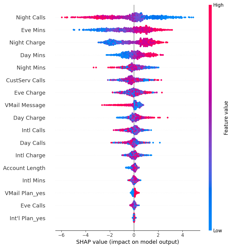
Some quick insights:
The more clients call at night, the less likely they will churn.
The longer clients call in evening, the less likely they will churn.
The higher the billed cost is for nighttime calls, the less likely clients will churn.
Can barely tell how values of
Int'l Plan_yesare associated with churn behaviors.
6. Conclusion
Some quick results:
Although we didn’t achieve a better score, 96.1% accuracy comparing to 97.9%, we achieve it fast and we are happy to accept it.
Night Calls,Eve Mins, andNight Chargeare the most influencial in determining whether a customer will churn, and we studied how their values will affect the churn behaviors.